Moving!

I have moved this blog to wordpress.com. Please, do visit blancosilva.wordpress.com for the updated version. Thanks!

Super-Resolution Micrograph Reconstruction by Nonlocal-Means Applied to High-Angle Annular Dark Field Scanning Transmission Microscopy (HAADF-STEM)

We outline a new systematic approach to extracting high-resolution information from HAADF–STEM images which will be beneficial to the characterization of beam sensitive materials. The idea is to treat several, possibly many low electron dose images with specially adapted digital image processing concepts at a minimum allowable spatial resolution. Our goal is to keep the overall cumulative electron dose as low as possible while still staying close to an acceptable level of physical resolution. We wrote a letter indicating the main conceptual imaging concepts and restoration methods that we believe are suitable for carrying out such a program and, in particular, allow one to correct special acquisition artifacts which result in blurring, aliasing, rastering distortions and noise.

Below you can find a preprint of that document and a pdf presentation about this work that I gave in the SEMS 2010 meeting, in Charleston, SC. Click on either image to download.

The Nonlocal-means Algorithm

The nonlocal-means algorithm [Buades, Coll, Morel] was designed to perform noise reduction on digital images, while preserving the main geometrical configurations, as well as finer structures, details and texture. The algorithm is consistent under the condition that one can find many samples of every image detail within the same image.

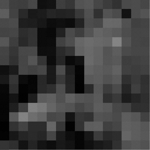
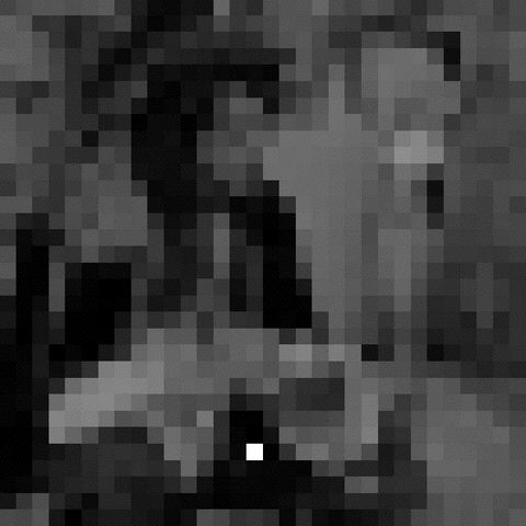
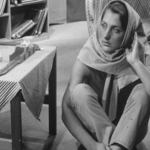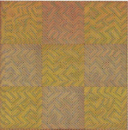
Barbara	Noise added, std=30	Denoised image, h=93

The algorithm has the following closed form: Given a finite grid $\Lambda \subset \mathbb{Z}^2$ of the form $\Lambda = \Omega \cap \mathbb{Z}^2$ for some compact set $\Omega \subset \mathbb{R}^2$, a signal $f \in L_2(\Lambda,\mathbb{R}^+)$, and a family of windows $\{ \mathcal{R}_k \}_{k \in \Lambda}$ satisfying the conditions

1. $k \in \mathcal{R}_k$ for all $k \in \Lambda$.
2. If $j \in \mathcal{R}_k$, then $k \in \mathcal{R}_j$,

the nonlocal-means operator $\operatorname{NL}_h\colon \ell_2(\Lambda,\mathbb{R}) \to \ell_2(\Lambda,\mathbb{R})$ with filtering parameter $h>0$, is defined by

\[\operatorname{NL}_h f(k) = \sum_{j \in \Lambda} \omega_h(j,k) f(j),\]

where the weights $\{ \omega_h(j,k) \}_{j,k \in \Lambda}$ are defined by

\[\omega_h(j,k) = \frac{ \exp \bigg( -\frac{\left\lVert f(\mathcal{R}_j) - f(\mathcal{R}_k) \right\rVert_{2,a}^2}{h^2} \bigg) }{ \sum_{j \in \Lambda} \exp \bigg( - \frac{\left\lVert f(\mathcal{R}_j) - f(\mathcal{R}_k) \right\rVert_{2,a}^2}{h^2} \bigg)}.\]

Here, $f(\mathcal{R})$ denotes a patch of the image $f$ supported on the window $\mathcal{R}$.

Notice that the similarity check between patches is nothing but a simple Gaussian weighted Euclidean distance, which accounts for difference of grayscales alone. Efros and Leung prove that this distance is a reliable measure for the comparison of texture patches, and at the same time copes very well with additive white noise; in particular, if $f$ and $g$ are respectively the noisy and original images, and $\sigma^2$ is the noise variance, then the most similar patches in the noisy image are also expected to be the most similar in the original:
\[ \mathbb{E} \left\lVert f(\mathcal{R}_j) - f(\mathcal{R}_k) \right\rVert_{2,a}^2 = \left\lVert g(\mathcal{R}_j) - g(\mathcal{R}_k) \right\rVert_{2,a}^2 + 2\sigma^2 .\]

The hunt for a Bellman Function.

I presented an introduction to Bellman Functions for the USC Math Dept Analysis Seminar in September 2008. This is a beautiful and powerful mathematical technique in Harmonic Analysis that allows, among other things, to prove very complicated inequalities in the theory of Singular Integral Operators, without using much of the classical machinery in this field. The Bellman function was the tool that allowed their creators (Fedor Nazarov and Sergei Treil) to crack the problem of weighted norm inequalities with matrix weights for the case $\boldsymbol{p} \neq \boldsymbol{2}$ and finally solve it completely. Copies of the original paper can be found at the authors' pages; e.g. [www.math.brown.edu/~treil/papers/bellman/bell3.ps] (notice the postscript file is huge, as the article has more than 100 pages). Let me illustrate the use of Bellman functions to solve a simple problem:

Dyadic-$\boldsymbol{L}_\mathbf{2}(\mathbb{R})$ version of the Carleson Imbedding Theorem Let $\mathcal{D}$ be the set of all dyadic intervals of the real line. Given a function $f \in L_1^{\text{loc}}(\mathbb{R})$, consider the averages $\langle f \rangle_I = \lvert I\rvert^{-1} \int_I f$, on each dyadic interval $I \in \mathcal{D}$. Let $\{ \mu_I \geq 0 \colon I \in \mathcal{D} \}$ be a family of non-negative real values satisfying the Carleson measure condition—that is, for any dyadic interval $I \in \mathcal{D}$, \[\sum_{J \subset I, J~\text{dyadic}} \mu_J \leq \lvert I \rvert.\]Then, there is a constant $C>0$ such that for any $f \in L_2(\mathbb{R})$,\[\sum_{ I \in \mathcal{D} } \mu_I \lvert \langle f \rangle_{I} \rvert^2 \leq C \lVert f \rVert_{L_2(\mathbb{R})}^2\]

Fix a dyadic interval $I \in \mathcal{D}$, and a vector $(x_1, x_2, x_3) \in \mathbb{R}^3$. Consider all families $\{\mu_I \colon I \in \mathcal{D} \}$ satisfying the Carleson condition $$\frac{1}{\lvert J \rvert} \sum_{K \subset J} \mu_{K} \leq 1, \text{ for all }J \in \mathcal{D}$$ and such that

(eq1)

$\displaystyle{\frac{1}{\lvert I \rvert} \sum_{J \subset I} \mu_J = x_1}$.

Also, consider all functions $f \in L_2(\mathbb{R})$ for which the following quantities are fixed:

(eq2)

$\displaystyle{\langle f^2 \rangle_I = \frac{1}{\lvert I \rvert} \int_I f^2 = x_2,\qquad \langle f \rangle_I = \frac{1}{\lvert I \rvert} \int_I f = x_3}$

If we believe that the Theorem is true, then the quantity $$\mathcal{B}(x_1,x_2,x_3)=\frac{1}{\lvert I \rvert} \sup \bigg\{ \sum_{J \subset I} \mu_J \langle f \rangle^2_J \colon f, \{ \mu_I \} \text{ satisfy }(eq1),(eq2) \bigg\}$$is finite and, moreover, satisfies the inequality $\mathcal{B}(x_1,x_2,x_3) \leq C x_2$. Since $\mathcal{B}(x_1,x_2,x_3)$ does not depend on the choice of an interval $I \in \mathcal{D}$, we obtain a function of three real variables; this is the Bellman function associated with the Carleson Imbedding Theorem. Notice that:

1. The domain of $\mathcal{B}$ is the set \[\{ (x_1, x_2, x_3) \in \mathbb{R}^3 \colon 0 \leq x_1 \leq 1, x_3^2 \leq x_2 \}.\]
2. For each $(x_1,x_2,x_3)$ in the domain of $\mathcal{B}$, it is \[0 \leq \mathcal{B}(x_1, x_2, x_3) \leq C x_2.\]
3. If $0 \leq \lambda \leq x_1$, then \[ \mathcal{B}(x_1, x_2, x_3)\geq \lambda x_2^2 + \frac{1}{2} \big\{ \mathcal{B}(x_1^+, x_2^+, x_3^+) + \mathcal{B}(x_1^-, x_2^-, x_3^-)\big\}\] whenever the triples $(x_1,x_2,x_3)$, $(x_1^+,x_2^+,x_3^+)$ and $(x_1^-,x_2^-,x_3^-)$ belong to the domain and \[\begin{gather} x_1 = \frac{1}{2}(x_1^+ + x_1^-) + \lambda, \\ x_2 = \frac{1}{2}(x_2^+ + x_2^-), \\ x_3 = \frac{1}{2}(x_3^+ + x_3^-). \end{gather}\]

The entire machine can be run backward: if we have any function $\mathcal{B}$ of three real variables that satisfies properties 1—3, the proof of the Theorem follows immediately. The key property 3 is not very pleasant to verify. Fortunately, this condition can be replaced by "infinitesimal" conditions (conditions on derivatives), which are easier to check: If $x_1 = \frac{1}{2}(x_1^+ + x_1^-)$, $x_2 = \frac{1}{2}(x_2^+ + x_2^-)$ and $x_3 = \frac{1}{2}(x_3^+ + x_3^-)$, and all triples are in the domain of $\mathcal{B}$, then the key property 3 implies the concavity of $\mathcal{B}$: $$ \mathcal{B}(x_1,x_2,x_3) \geq \frac{1}{2} \big\{ \mathcal{B}(x_1^+,x_2^+,x_3^+) + \mathcal{B}(x_1^-,x_2^-,x_3^-)\big\} $$and furthermore,

(eq3)

$\displaystyle{d^2 \mathcal{B} \leq 0, \qquad \frac{\partial \mathcal{B}}{\partial x_1} \geq x_3^2}$

Notice that condition 3 is equivalent to (eq3). The following function satisfies 1, 2 and (eq3), and thus the Theorem is proven for $C=4$. $$\mathcal{B}(x_1, x_2, x_3) = 4\bigg( x_2 - \frac{x_3^2}{1+x_1}\bigg)$$

Mathematics Genealogy Project

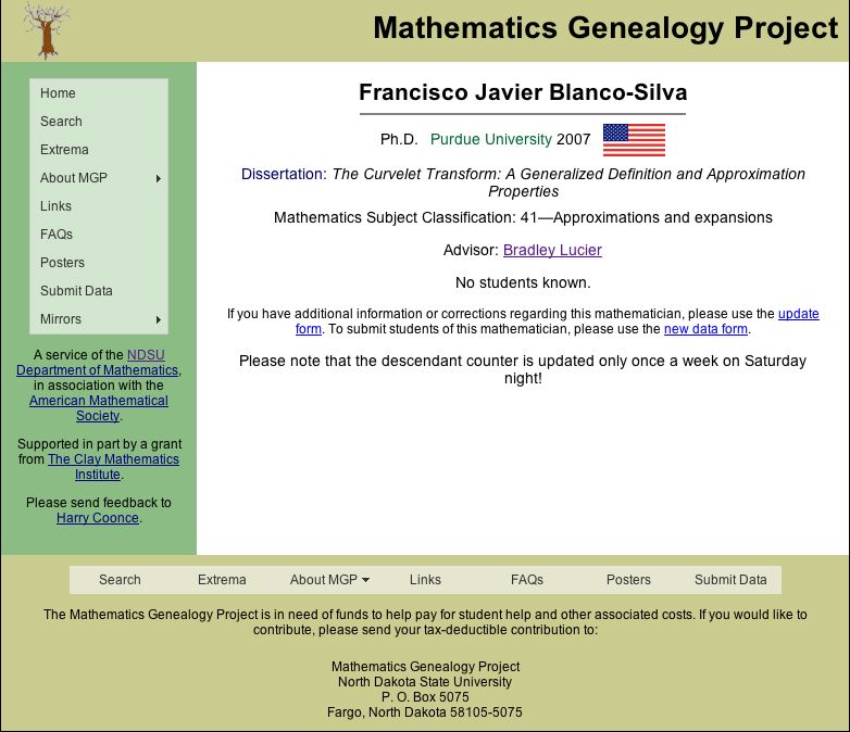
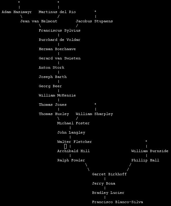
I traced my mathematical lineage back into the XVII century at The Mathematics Genealogy Project. Imagine my surprise when I discovered that my ancestors started as physicians, chemists, physiologists and anatomists.

There is some "blue blood" in my family: Garrett Birkhoff, William Burnside (both algebrists), and Archibald Hill, who shared the 1922 Nobel Prize in Medicine for his elucidation of the production of mechanical work in muscles. He is regarded, along with Hermann Helmholtz, as one of the founders of Biophysics.

Thomas Huxley (a.k.a. "Darwin's Bulldog", biologist and paleontologist) participated in that famous debate in 1860 with the Lord Bishop of Oxford, Samuel Wilberforce. This was a key moment in the wider acceptance of Charles Darwin's Theory of Evolution.

There are some hard-core scientists in the XVIII century, like Joseph Barth and Georg Beer (the latter is notable for inventing the flap operation for cataracts, known today as Beer's operation).

My namesake Franciscus Sylvius, another professor in Medicine, discovered the cleft in the brain now known as Sylvius' fissure (circa 1637). One of his advisors, Jan Baptist van Helmont, is the founder of Pneumatic Chemistry and disciple of Paracelsus, the father of Toxicology (for some reason, the Mathematics Genealogy Project does not list him in my lineage, I wonder why).

Click on either image for a larger version.

Presentation: The Hitchhiker's Guide to the…

This is a very gentle exposition to the transforms of Hilbert, Fourier and Wavelet, with obvious application to the construction of the Dual-Tree Complex Wavelet Transform. It was meant to be an introduction to my current research for the students in the SIAM seminar, and thus no previous background in Approximation Theory or Harmonic Analysis is needed to follow the slides. Everyone with knowledge of integration should be able to understand and enjoy the ideas behind this beautiful topic.

Click on the slide below to retrieve a pdf file with the presentation.

Presentation: Hilbert Transform Pairs of Wavelets

Now in the stage of the Approximation Theory Seminar, I presented a general overview of the work of Selesnick and others towards the design of pairs of wavelet bases with the "Hilbert Transform Pair property". Click on the image below to retrieve a pdf file with the slides.

Presentation: The Dual-Tree Complex Wavelet Transform

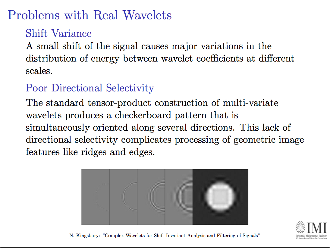
In the first IMI seminar, I presented an introduction to the survey paper "The Dual-Tree Complex Wavelet Transform", by Selesnick, Baraniuk and Kingsbury. It was meant to be a (very) basic overview of the usual techniques of signal processing with an emphasis on wavelet coding, an exposition on the shortcomings of real-valued wavelets that affect the work we do at the IMI, and the solutions proposed by the three previous authors. In a subsequent talk, I will give a more mathematical (and more detailed) account on filter design for the dual-tree C(omplex)WT. Click on the image below to retrieve a pdf version of the presentation.

Presentation: Curvelets and Approximation Theory

Find below a set of slides that I used for my talk at the IMA in the Thematic Year on Mathematical Imaging. On them, there is a detailed construction of my generalized curvelets, some results by Donoho and Candès explaining their main properties, and a bunch of applications to Imaging. Click on the slide below to retrieve the pdf file with the presentation.

Poster: Applications of the Curvelet Transform to Imaging

(Click on image for pdf file)

Poster: Curvelets vs. Wavelets (Mathematical Models of Natural Images)

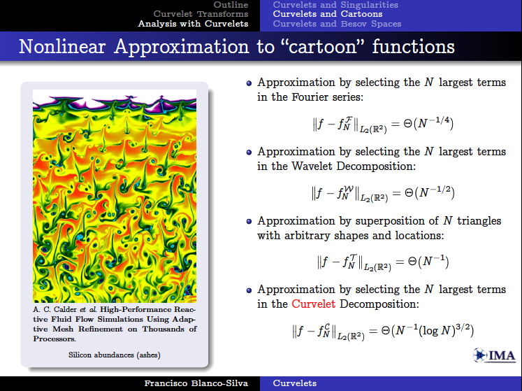
Together with Professor Bradley J. Lucier, we presented a poster in the Workshop on Natural Images during the thematic year on Mathematical Imaging at the IMA. We experimented with wavelet and curvelet decompositions of 24 high quality photos from a CD that Kodak® distributed in the late 90s. All the experiment details and results can be read in the file Curvelets/talk.pdf.

The computations concerning curvelet coefficients were carried out in Matlab, with the Curvelab 2.0.1 toolbox developed by Candès, Demanet, Donoho and Ying. The computations concerning wavelet coefficients were performed by Professor Lucier's own codes.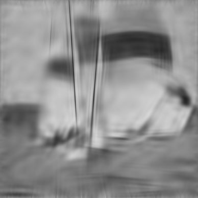

Wavelet Coefficients

To aid in my understanding of wavelets, during the first months I started studying this subject I wrote a couple of scripts to both compute wavelet coefficients of a given pgm gray-scale image (the decoding script), and recover an approximation to the original image from a subset of those coefficients (the coding script). I used OCaml, a multi-paradigm language: imperative, functional and object-oriented.

The decoding script uses the easiest wavelets possible: the Haar functions. As it was suggested in the article "Fast wavelet techniques for near-optimal image processing", by R. DeVore and B.J. Lucier, rather than computing the actual raw wavelet coefficients, one computes instead a related integer value (a code). The coding script interprets those integer values and modifies them appropriately to obtain the actual coefficients. The storage of the integers is performed using Huffman trees, but I used a very simple one, not designed for speed or optimization in any way.

Following a paper by A.Chambolle, R.DeVore, N.Y.Lee and B.Lucier, "Non-linear wavelet image processing: Variational problems, compression and noise removal through wavelet shrinkage", these scripts were used in two experiments later on: computation of the smoothness of an image, and removal of Gaussian white noise by the wavelet shrinkage method proposed by Donoho and Johnstone in the early 90's.

Progressive reconstruction of a grey-scale image of size 1024 x 1024 with the largest (in absolute value) 2ⁿ coefficients, n = 1,2,…,8

Notes on Approximation Theory

I created the following notes for my Advanced Topics Exam: They are mostly based on ideas from both Ronald DeVore's "Nonlinear Approximation", and DeVore & Popov's "Interpolation of Besov Spaces." These notes pretend to serve as a tool to understand the problems that Constructive Approximation solve, most of the background results in this Theory, and the intimate relationship with other branches of Mathematics (for example, showing how working within a purely "Approximation Theory" scope, one can find Interpolation Spaces between Besov Spaces [Interpolation of Operators]).

• HTML version: AT2/root.html
• PDF version: AT2/root.pdf

Modeling the Impact of Ebola and Bushmeat Hunting on Western Lowland

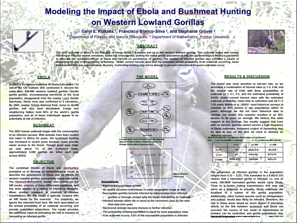
In May 2003, together with fellow Mathematician Stephanie Gruver, Statistician Young-Ju Kim, and Forestry Engineer Carol Rizkalla, we worked on this little project to apply ideas from Dynamical Systems to an epidemiology model of the Ebola hemorrhagic fever in the Republic of Congo. The manuscript ebola/root.pdf is a first draft, and contains most of the mathematics behind the study. Carol worked in a less-math-more-biology version: ebola/Ecohealth.pdf "Modeling the Impact of Ebola and Bushmeat Hunting on Western Lowland Gorillas," and presented it to EcoHealth, where it has been published (June 2007). She also prepared a poster for the Sigma-Xi competition: Click on the image below to retrieve a PowerPoint version of it.

Kinetics on Networks of Enzymatic Reactions

I worked in a project of analysis and simulation of kinetics on networks of enzymatic reactions for a course in BioInformatics. An example: The graph depicted here represents the RKIP network. Substrates, enzymes and substrate/enzyme complexes are represented by numbered circles, while rate constants are represented by numbered squares. As a straight-forward application of dynamical systems and numerical solution of systems of differential equations, I wrote a very simple script in Python which allows a user to input the name of an enzyme, and obtain:

1. All networks of chemical reactions in which the input enzyme is present.
2. The corresponding (biochemically-correct) systems of algebraic-differential equations expressing the rate of change of the compounds with respect to time.
3. Solution to those systems (after user inputs also a set of initial conditions for both the enzymes and substrates)
4. Visualization of the process by means of network graphs, plots of amount of chemical compounds with respect to time, etc

Click on the picture above to retrieve a brief report of the project. Find below a concise explanation, and a description of the database ENZYME, used for the online search of the networks:

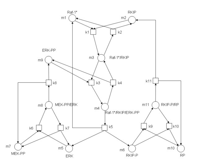
Consider the dynamics of a biochemical network of enzymatic reactions: given, from a database, a set of chemical reactions involving related enzymes, each of these take certain amounts of one or several compounds (substrate), and after the reaction, output one or several reactants (notice that the reaction can proceed in either way, depending mainly on the concentration of substrate and reactant). Notice also that both input and output of those reactions might be used by different enzymes in another related reactions. In this way, if we could “freeze” the reactions at any given time, and measure the concentration of each component being used in this network, we would be able to answer questions of the kind: “Which component decays faster?”, “when will the reactions stop?” (provided the enzymes don’t “die”), “what are the initial concentrations that produce certain phenomena?”, etc. All these can be answered from a “Dynamical Systems” point of view. Each of the chemical reactions offer a special differential equation involving not only the concentration of the components, but also the concentration of the enzyme and a few more parameters. This differential equations are constrained by the fact that none of the concentrations (=variables) can drop below zero. These are just a small example of the so-called differential-algebraic systems of equations. Given a network of chemical reactions produced by enzymes, included initial concentrations of components and enzymes, model the dynamical behavior using a differential-algebraic system of equations. The outputs will be, for instance, graphs of the change in the concentration of substrate or reactant A with respect to time. Of great interest is also the procedure of finding the network itself. For instance, given a certain protein, find all known enzymatic reactions related to the manipulation of this protein. Arrange them in a network, and study its dynamical properties. The first part involves taking information from a database, and a second part involves manipulating that information to obtain the desired network. ENZYME is a repository of information relative to the nomenclature of enzymes. It is primarily based on the recommendations of the Nomenclature Committee of the International Union of Biochemistry and Molecular Biology (IUBMB) and it describes each type of characterized enzyme for which an EC (Enzyme Commission) number has been provided. It contains the following data:

1. EC number
2. Recommended name
3. Alternative names (if any)
4. Catalytic activity
5. Cofactors (if any)
6. Pointers to the SWISS-PROT entry that corresponds to the enzyme (if any)
7. Pointers to diseases associated with a deficiency of the enzyme (if any)

The main source for the data in the ENZYME database comes from recommendations of the Nomenclature Committee of the IUBMB.

Triangulations

As part of a project developed by Professor Bradley J. Lucier, to code a PDE solver written in Scheme, I worked in some algorithms to perform "good triangulations" of polygons with holes ("good triangulations" meaning here, those where all the triangles have their three angles as close to 60º as possible). I obtained the necessary theoretical background and coding strategies from the following references:

• Mark de Berg et al., "Computational Geometry by Example."
• Francis Chin and Cao An Wang, "Finding the Constrained Delaunay Triangulation and Constrained Voronoi Diagram of a simple Polygon in Linear Time."
• Joseph O'Rourke, "Computational Geometry in C."
• Jim Ruppert, "A Delaunay Refinement Algorithm for Quality 2-dimensional Mesh Generation."

Mechanical Geometry Theorem Proving

In 1977, Professor Wen-Tsun Wu succeeded in developing a method of mechanical geometry theorem proving. This method has been applied to prove or even discover hundreds of non-trivial difficult theorems in elementary and differential geometries on a computer in an almost trivial manner. Usign Ritt's differential algebra, Wu established a method for solving algebraic and differential equations by transforming an equation system in the general form to equation systems in triangular form. This is the Ritt-Wu decomposition algorithm, that later on was shown to be equivalent to perform a series of operations on ideals, very easily carried out by means of Gröbner basis manipulation.

I wrote a script in MAPLE to perform evaluations of the validity of some simple theorems in Euclidean Geometry, and wrote a small paper (in Spanish) on one of my findings, that was published in Bol. Asoc. Prof. Puig Adams, in October'99: "Sobre demostración automática de un problema geométrico".

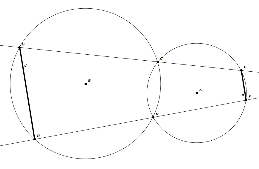
The example I cover in that short article can be seen below. Given: Circles A, B that intersect each other in points C and D, and given points E, F in circle A, consider line a through E and C, and line b through F and D. The intersections of line a with circle B are C and G. The intersections of line b with circle B are D and H. Consider the segments c (connecting E with F) and d (connecting G with H). To prove: Segments c and d are parallel.